300
cd/klm
30°
24 230
60°
30°
0°
30°
60°
cd/klm
500
1000
77 584
ß= 32°/88°
60°
30°
0°
30°
60°
cd/klm
600
1200
84 503
ß= 27°/76°
¯E
lx
84 503
LED
m
640
480
320
160
4
0
4
8
800
2
6
10
14
18
16 m
18 m
8 m
•
•
•
•
lx
84 503
LED
m
640
480
320
160
4
0
4
8
800
2
6
10
14
18
¯E
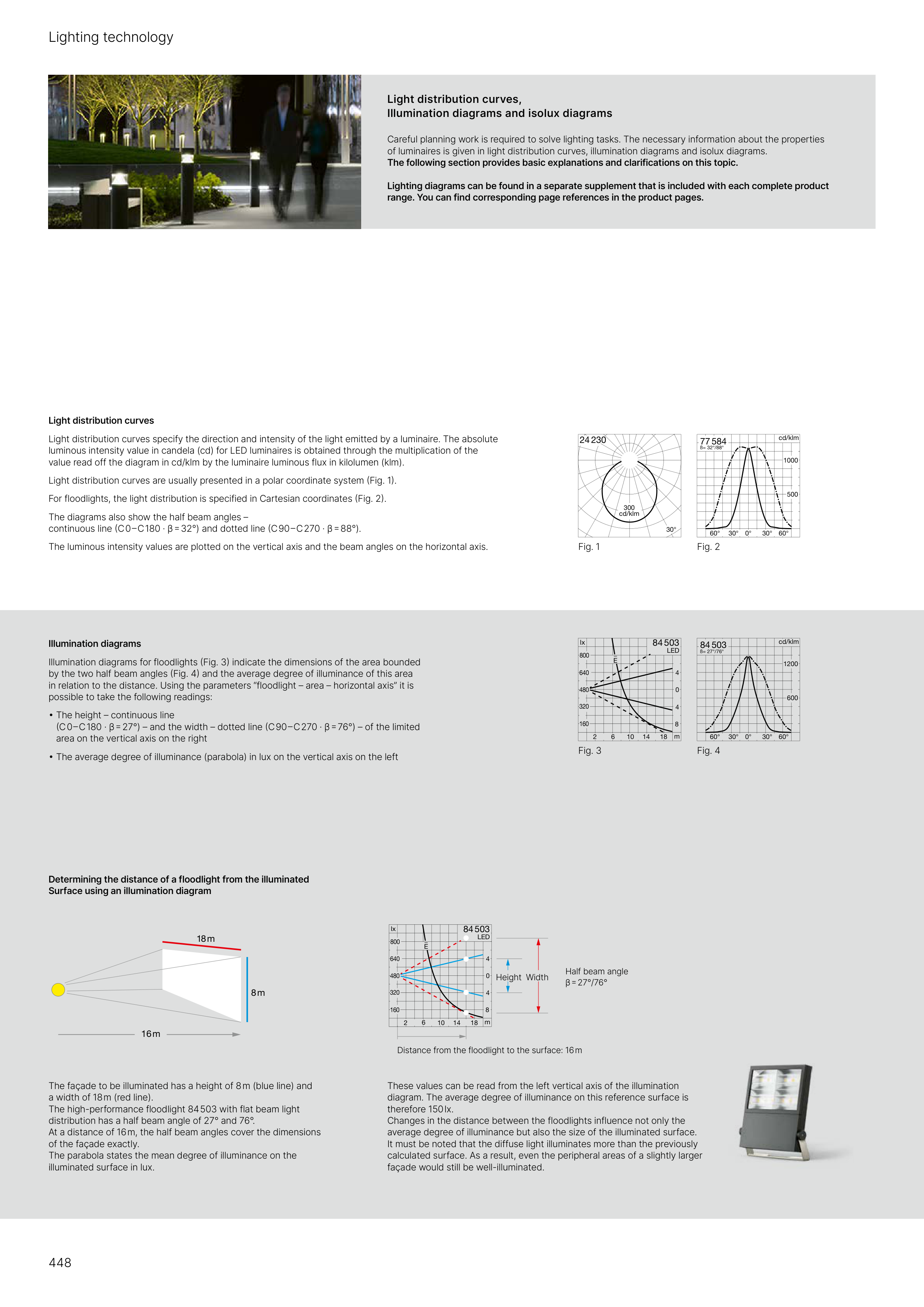
The façade to be illuminated has a height of 8 m (blue line) and
a width of 18 m (red line).
The high-performance floodlight 84 503 with flat beam light
distribution has a half beam angle of 27° and 76°.
At a distance of 16 m, the half beam angles cover the dimensions
of the façade exactly.
The parabola states the mean degree of illuminance on the
illuminated surface in lux.
These values can be read from the left vertical axis of the illumination
diagram. The average degree of illuminance on this reference surface is
therefore 150 lx.
Changes in the distance between the floodlights influence not only the
average degree of illuminance but also the size of the illuminated surface.
It must be noted that the diffuse light illuminates more than the previously
calculated surface. As a result, even the peripheral areas of a slightly larger
façade would still be well-illuminated.
Half beam angle
β = 27°/76°
Distance from the floodlight to the surface: 16 m
Height Width
Determining the distance of a floodlight from the illuminated
Surface using an illumination diagram
Illumination diagrams
Illumination diagrams for floodlights (Fig. 3) indicate the dimensions of the area bounded
by the two half beam angles (Fig. 4) and the average degree of illuminance of this area
in relation to the distance. Using the parameters “floodlight – area – horizontal axis” it is
possible to take the following readings:
• The height – continuous line
(C 0 – C 180 · β = 27°) – and the width – dotted line (C 90 – C 270 · β = 76°) – of the limited
area on the vertical axis on the right
• The average degree of illuminance (parabola) in lux on the vertical axis on the left
Light distribution curves
Light distribution curves specify the direction and intensity of the light emitted by a luminaire. The absolute
luminous intensity value in candela (cd) for LED luminaires is obtained through the multiplication of the
value read off the diagram in cd/klm by the luminaire luminous flux in kilolumen (klm).
Light distribution curves are usually presented in a polar coordinate system (Fig. 1).
For floodlights, the light distribution is specified in Cartesian coordinates (Fig. 2).
The diagrams also show the half beam angles –
continuous line (C 0 – C 180 · β = 32°) and dotted line (C 90 – C 270 · β = 88°).
The luminous intensity values are plotted on the vertical axis and the beam angles on the horizontal axis.
Fig. 3
Fig. 4
Fig. 2
Fig. 1
Light distribution curves,
Illumination diagrams and isolux diagrams
Careful planning work is required to solve lighting tasks. The necessary information about the properties
of luminaires is given in light distribution curves, illumination diagrams and isolux diagrams.
The following section provides basic explanations and clarifications on this topic.
Lighting diagrams can be found in a separate supplement that is included with each complete product
range. You can find corresponding page references in the product pages.
Lighting technology
448